
What Are Bollinger Bands?
Bollinger Bands are a technical analysis indicator built to measure price movement against changing market volatility. Created by John Bollinger in the 1980s, this trademark tool remains a staple on modern charting platforms used by traders worldwide.
At its core, a Bollinger Bands definition describes a statistical chart overlay plotted directly onto price. It combines a moving average with standard deviation bands to visually frame how far price typically strays from its recent average value.
Unlike fixed support and resistance lines, Bollinger Bands form a dynamic price envelope. This envelope expands and contracts automatically, adjusting to real market conditions rather than relying on arbitrary, manually drawn levels that traders must constantly redraw.
As a volatility indicator, the tool does not predict direction on its own. Instead, it contextualizes price by showing whether current movement is unusually large or small relative to recent historical behavior.
Many traders first encounter Bollinger Bands as simple moving average bands layered on a candlestick chart. Understanding the mechanics behind that visual, however, requires looking closely at the three components that construct every band.
The Three Components of a Bollinger Band
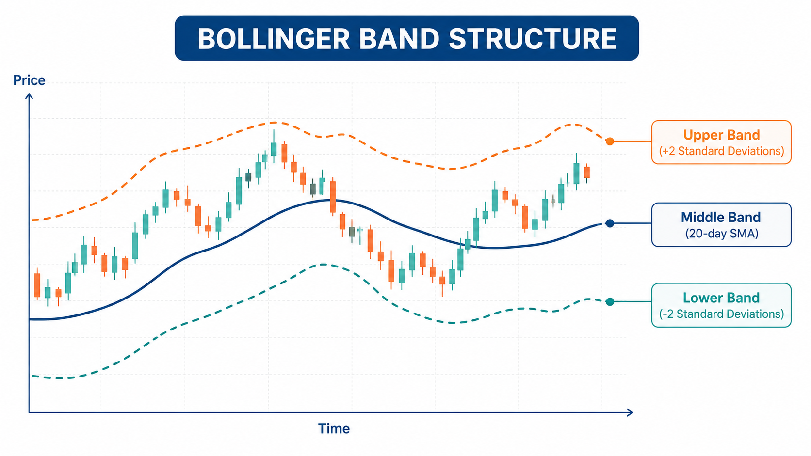
Every Bollinger Band setup consists of three distinct lines working together within a single band structure. These lines are the middle band, the upper band, and the lower band, each serving a specific analytical purpose.
The middle band is simply a simple moving average, most commonly calculated using a 20-period SMA. This line smooths out short-term price noise and represents the average closing price over the selected lookback window.
The upper band sits above the middle band, calculated by adding a multiple of standard deviation to the moving average. It marks a statistically elevated price zone relative to recent average trading activity.
The lower band mirrors this process on the downside, subtracting the same standard deviation multiple from the middle line. Together, upper and lower bands form the outer edges of the price envelope.
Because standard deviation reacts to volatility, the space between these three lines is never fixed. When markets grow calmer or more turbulent, the entire band structure reshapes itself in response.
How Bollinger Bands Are Calculated (Formula)
Understanding the Bollinger Bands formula requires breaking the indicator into its underlying calculation steps. Each band is derived mathematically from price data, not drawn subjectively, which gives the indicator its analytical consistency.
The process begins with a moving average calculation, typically using a 20-day SMA of closing prices. This average becomes the baseline from which both outer bands are measured and adjusted.
Next, the standard deviation formula is applied to the same price data set. This figure quantifies how much individual closing prices deviate from that moving average across the chosen period.
The multiplier, usually set at two, is then applied to the standard deviation value. This scaled figure is added to produce the upper band formula and subtracted to produce the lower band formula.
Following this step by step calculation consistently allows traders to reproduce band values manually. Most charting software automates the math, but understanding the formula clarifies why bands widen and narrow.
The Formula Explained
The middle band formula is expressed simply as the moving average of closing prices over the chosen lookback period. Most platforms default to twenty periods unless a trader adjusts the setting manually.
From there, the upper band = SMA + 2 SD formula adds two standard deviations above that moving average line. This creates a statistical ceiling representing an elevated, though not impossible, price extreme.
Conversely, lower band = SMA − 2 SD subtracts the same amount below the average. The standard deviation calculation driving both formulas measures dispersion of prices around their mean value precisely.
Worked Example With Real Numbers
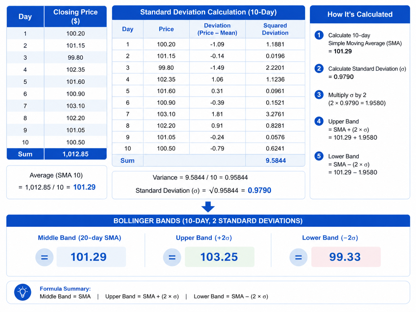
Consider a sample calculation using sample stock prices over a twenty-day window. Suppose the sample 20-day closing prices average out to a simple moving average of exactly $100.00 for illustration purposes.
Next, calculating standard deviation manually across those same twenty closing prices might yield a value of $2.00. This figure reflects how tightly or loosely the prices cluster around that $100.00 average.
Applying the formula through this step by step example, the upper band becomes $104.00, and the lower band becomes $96.00. This range visually represents typical price dispersion for that specific period.
How Bollinger Bands Work
Bollinger Bands function through a continuous cycle of volatility expansion and volatility contraction. When market activity intensifies, the bands widen; when trading calms down, the bands draw closer together again.
This behavior appears visually as band widening during volatile news events or earnings releases. Traders often watch for this expansion as a signal that price is moving with unusual force relative to recent norms.
Conversely, band narrowing reflects a quieter market phase where price trades within a tighter range. Periods of narrowing frequently precede larger moves, since volatility tends to alternate between calm and active phases.
Because the bands are statistically derived, prices touching either edge represent relative high and low prices rather than fixed value judgments. A touch simply means price sits near a statistical extreme for that period.
This dynamic structure supports a concept known as mean reversion, where price tends to gravitate back toward the middle band over time. The underlying price envelope logic treats the bands as adaptive, not static, boundaries.
Choosing Bollinger Band Settings for Different Trading Styles
The default settings for Bollinger Bands use a 20 period 2 standard deviations configuration on most charting platforms. This combination works reasonably well across many timeframes but is not universally optimal.
Traders focused on intraday settings often shorten the lookback period so the bands react faster to rapid price shifts. Day trading settings prioritize responsiveness over smoothness, given the compressed timeframes involved.
Swing trading settings typically retain something closer to the default configuration, balancing responsiveness with reliability. This middle-ground approach suits traders holding positions across several days rather than minutes or months.
Long-term investing settings usually stretch the lookback period further, filtering out short-term noise entirely. Position-oriented traders value smoother, more stable bands over highly reactive ones on shorter charts.
Beyond period length, adjusting standard deviation multiplier values also changes band sensitivity. Combined with timeframe customization and adjusting period length, these settings let traders tailor the indicator to their specific approach.
Settings for Short-Term / Day Trading
Short-term traders often reduce the lookback window toward a 10-period setting to capture faster price swings. This adjustment suits scalping approaches where positions last only minutes rather than hours or days.
On intraday charts, this shorter period produces faster reacting bands that respond quickly to sudden volatility shifts. The tradeoff is more frequent band touches, some of which may prove less reliable statistically.
Because faster bands generate more signals, day traders typically pair this setting with strict risk controls. Speed alone does not improve accuracy, so confirmation from price action remains genuinely important here.
Settings for Swing Trading
Swing traders generally favor the 20-period default setting because it balances responsiveness with statistical reliability. This period aligns naturally with common daily charts, matching roughly one calendar month of trading activity.
The standard 2 SD setting captures a wide enough range to filter minor noise while still highlighting meaningful price extremes. This configuration suits traders holding positions across several days to a few weeks.
Because swing trading timeframes sit between scalping and long-term investing, this default configuration often requires little adjustment. Many traders find the standard settings sufficient without further customization for typical swing strategies.
Settings for Long-Term Investing
Long-term investors often extend the lookback window toward a 50-period setting for a smoother, less reactive view. This adjustment suits weekly charts, where each data point represents several trading days of activity.
This longer setting supports position trading, where holding periods stretch across months rather than days or weeks. The extended timeframe naturally filters out short-term volatility that carries little relevance for longer horizons.
The primary benefit of this approach is smoothing out noise that would otherwise clutter a long-term perspective. Fewer false signals appear, though the tradeoff is slower responsiveness to sudden market shifts.
How to Use Bollinger Bands in Trading and Investing
Bollinger Bands support a range of applications within a broader trading strategy framework. Traders commonly use the indicator to assess overbought conditions and oversold conditions relative to recent price behavior.
One common application involves watching for price touching upper band or price touching lower band levels as potential turning points. These touches are observations, not automatic buy and sell signals, and require further context.
Bollinger Bands also assist with trend confirmation, helping traders distinguish a genuine uptrend from a downtrend based on how price interacts with the band structure over time.
Some traders incorporate the indicator when identifying possible entry and exit points, though most experienced users combine it with other analytical tools rather than relying on it in isolation.
Because markets behave differently across conditions, no single band-based signal works universally. The following subsections outline specific ways traders commonly interpret Bollinger Band behavior in practice.
Overbought and Oversold Signals
An upper band touch is sometimes read as a sign of a relative high price within recent trading history. Similarly, a lower band touch may indicate a relative low price for that same window.
These touches are frequently associated with a possible reversal signal, particularly within range-bound markets. Traders watching for a mean reversion trade often look for price to pull back toward the middle band.
However, band touches alone do not guarantee reversal, since strong trends can push price along a band edge repeatedly. Context, volume, and other confirming signals remain essential before acting on any single touch.
The Bollinger Band Squeeze (Volatility Breakout Strategy)
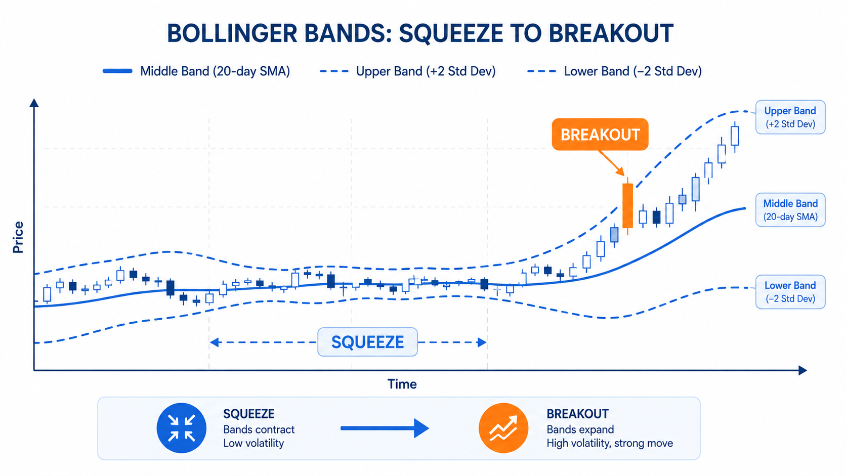
A band squeeze occurs during a low volatility period, when the upper and lower bands draw unusually close together. This volatility contraction often signals that the market is compressing before a potential larger move.
Traders monitoring a squeeze setup frequently reference the BandWidth indicator to quantify how tight the bands have become numerically. This tool helps identify unusually narrow conditions that may precede a breakout signal.
Because a squeeze does not indicate direction, many traders wait for volume confirmation before acting. Observing the direction of breakout alongside rising volume helps distinguish a genuine move from a false start.
Walking the Bands (Trend Confirmation)
During a strong uptrend, price sometimes exhibits price hugging upper band behavior for an extended stretch, a pattern often called riding the band. This persistent contact reflects sustained buying pressure rather than exhaustion.
The same concept applies inversely during a strong downtrend, where price hugging lower band conditions can persist across multiple sessions. In both cases, repeated touches do not automatically signal reversal.
This behavior offers a form of trend strength confirmation, since sustained band contact often reflects momentum rather than an imminent turning point. Traders use this pattern to avoid premature reversal assumptions.
W-Bottoms and M-Tops
A double bottom pattern, sometimes called a W-bottom, describes two successive lows near the lower band where the second low holds above the first. This structure can suggest waning downside momentum.
Conversely, a double top pattern, or M-top, forms when two peaks near the upper band appear with the second failing to exceed the first significantly. This may indicate weakening upward momentum.
John Bollinger himself documented these formations as part of broader pattern recognition work built around the indicator. Reversal pattern confirmation typically requires additional context beyond band position alone.
%B and BandWidth: Advanced Bollinger Band Indicators
Beyond the basic bands, two derived tools extend their analytical usefulness considerably. The %B indicator formula expresses exactly where price sits relative to the upper and lower bands numerically.
A %B reading near one suggests price sits close to the upper band, while a reading near zero suggests proximity to the lower band. This offers precise quantifying position within bands rather than visual estimation.
The BandWidth indicator formula, by contrast, measures the distance between the upper and lower bands as a percentage of the middle band. This produces a dedicated volatility measurement tool independent of price direction.
Both indicators support more structured system building, allowing traders to define specific numeric thresholds rather than relying purely on visual judgment of chart patterns.
Together, %B and BandWidth transform Bollinger Bands from a purely visual overlay into a genuine pattern recognition tool capable of supporting quantitative, rules-based analysis approaches.
Combining Bollinger Bands With Other Technical Indicators
Bollinger Bands are rarely used in complete isolation by experienced technical analysts. Many traders pair band signals with RSI confirmation, checking whether momentum readings align with apparent overbought or oversold conditions.
MACD confirmation offers another layer of validation, helping traders assess whether momentum direction supports a potential band-based signal before considering any action within their broader strategy.
Volume confirmation remains particularly important, since price moves accompanied by strong volume tend to carry more statistical weight than those occurring on comparatively thin trading activity.
A moving average crossover on a separate timeframe can further support trend-related conclusions drawn from band behavior, adding another independent data point to the overall analysis.
This layered approach reflects a broader multi-indicator strategy philosophy, aimed specifically at avoiding false signals that might otherwise arise from relying on any single indicator alone.
Bollinger Bands vs. Other Volatility Indicators
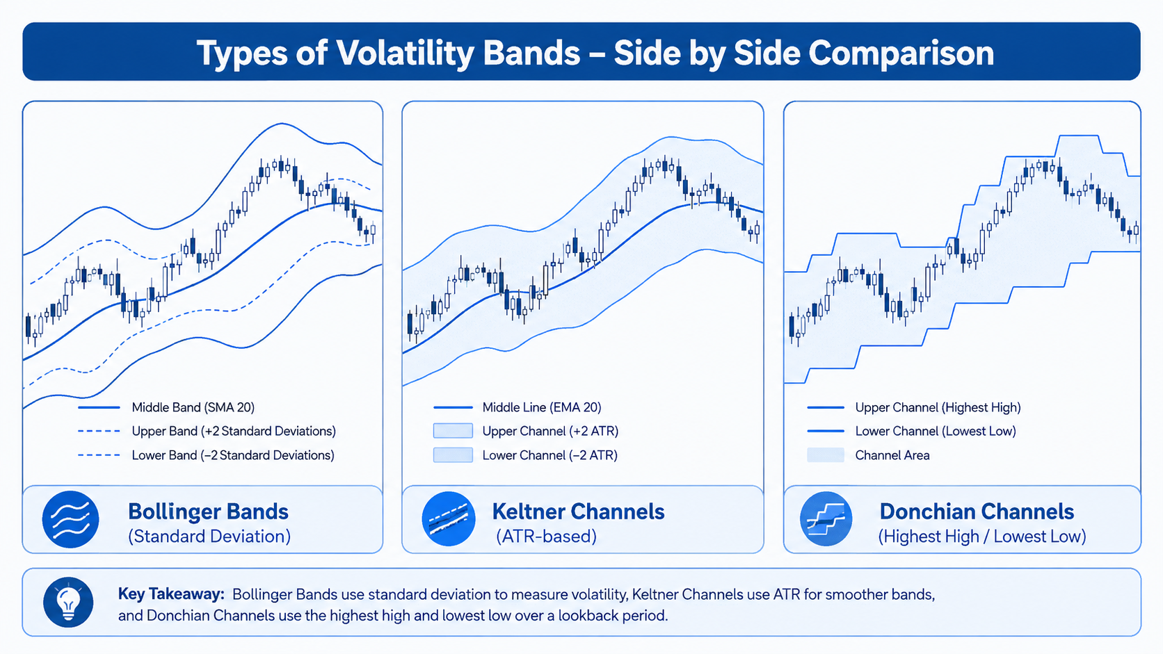
Bollinger Bands are one of several tools designed to measure market volatility, and a Keltner Channels comparison highlights key structural differences. Keltner Channels use average true range instead of standard deviation.
A Donchian Channels comparison reveals another contrast, since Donchian Channels simply track the highest high and lowest low over a set period, without any statistical smoothing applied.
ATR bands comparison studies often focus on the underlying calculation method itself, framing the distinction as standard deviation vs average true range approaches to measuring price volatility numerically.
Each method produces visually similar band structures but reacts differently to sudden price spikes, since standard deviation is more sensitive to extreme outlier values than average true range.
Deciding when to use which indicator often depends on personal preference and market conditions, since no single volatility tool consistently outperforms the others across every scenario.
Limitations and Common Mistakes When Using Bollinger Bands
Like any technical tool, Bollinger Bands carry inherent limitations worth understanding clearly. Because the indicator relies on moving averages, it functions as a lagging indicator, reacting to price rather than predicting it.
This lag can produce false signals, particularly in choppy or sideways markets where price repeatedly touches the bands without any meaningful follow-through in either direction.
Bollinger Bands are explicitly not a standalone strategy on their own. Over-reliance on bands without supporting context frequently leads traders toward premature or poorly timed decisions.
Whipsaw markets present a particular challenge, since rapid direction changes can trigger multiple conflicting signals within a short period, undermining confidence in any single band-based reading.
A common mistake involves misreading band touches as automatic signals rather than observations requiring further analysis. Additionally, backtesting limitations mean historical performance never guarantees similar future indicator behavior.
Frequently Asked Questions
What is a good Bollinger Band setting for day trading?
Many day traders experiment with 10-period Bollinger Bands on intraday charts to capture faster price movement. These tighter scalping settings increase responsiveness but may also generate more frequent signals.
Do Bollinger Bands work on all assets, including crypto and forex?
Crypto Bollinger Bands and forex Bollinger Bands function using the same underlying formula applied to stocks, commodities, and futures. Asset applicability is broad, though volatility characteristics differ across markets.
What does it mean when Bollinger Bands are very narrow?
Narrow bands typically reflect a squeeze condition tied to unusually low volatility. Traders often treat this as breakout anticipation, watching closely for a subsequent expansion in either direction.
Is it a buy signal when price touches the lower Bollinger Band?
A lower band touch alone is not a reliable signal. It may reflect oversold conditions, but without confirmation needed, it can also represent a false signal during strong downtrends.
What’s the difference between Bollinger Bands and moving averages?
The moving average vs Bollinger Bands distinction centers on volatility. An SMA shows only average price, while Bollinger Bands add a volatility dimension through upper and lower boundaries.
Can Bollinger Bands be used alone as a complete trading strategy?
Bollinger Bands are generally not treated as a standalone strategy. Most traders rely on indicator confirmation, sound risk management, and combining indicators rather than a single tool alone.
Who created Bollinger Bands and when?
John Bollinger developed the indicator during the 1980s, drawing on years of technical analysis history. The tool remains a registered trademark associated with his original methodology.
What is the difference between Bollinger Bands and Keltner Channels?
Keltner Channels rely on ATR rather than standard deviation for width calculation. Some traders use a squeeze indicator combination of both tools together for added confirmation.