Discounted Cash Flow Valuation: How the DCF Method Works

What Is Discounted Cash Flow (DCF) Valuation?

Discounted cash flow valuation estimates a company’s intrinsic value by projecting its future cash flows and converting each projected amount into present value today, using a chosen discount rate, an important point for anyone building financial models.

It reflects the time value of money, since a dollar received later is worth less than one received now, given inflation and the opportunity to invest that money elsewhere, a detail that matters for accurate valuation work.

Investors and analysts rely on this income approach for business valuation because it looks closely at what a company actually generates in cash, not simply what the market currently pays for shares.

This makes DCF analysis central to serious investment valuation work across industries and company sizes, from early startups to large established public corporations with long operating histories, which analysts must weigh carefully in practice.

The valuation method matters because prices in public markets can drift from underlying fundamentals for long stretches, and a carefully built DCF model gives investors an independent reference point, a factor that shapes the final valuation outcome.

The Time Value of Money Explained

The time value of money is the idea that cash available today is worth more than the exact same amount received later, because money can grow when invested wisely, something every serious financial analyst should understand well.

Opportunity cost also plays a central role here. Holding cash without putting it to work means missing potential returns elsewhere, so investors always weigh what could have been earned instead, a nuance that affects how the model performs.

Discounting converts future dollar amounts back into today’s terms using a required rate of return, one that reflects inflation, general risk, and the natural preference for money now over later, which directly influences the credibility of the result.

DCF vs. Book Value vs. Market Value

Book value reflects what a company’s assets are officially worth on its accounting records, after subtracting total liabilities, and it relies heavily on historical cost rather than future potential, a point worth remembering when reviewing any model.

Market value, in contrast, reflects what investors are currently willing to pay for a company’s outstanding shares, a price often driven by sentiment, momentum, or breaking news rather than fundamentals, which can meaningfully change the final valuation figure.

DCF valuation aims for a clearer intrinsic value vs market price comparison, weighing computed worth against current enterprise value in the market, labeling the gap as overvalued or undervalued, an idea central to sound financial decision-making overall.

The DCF Formula Explained

The DCF formula sums the present value of every projected cash flow across the entire forecast period, then adds the separately discounted terminal value to reach one combined total, a consideration that shapes how investors read the output.

In its simplest form, the present value formula divides each future cash flow by a growing discount factor, one that expands with every additional year further into the future, which underscores why careful assumptions matter so much.

Written formally, the NPV formula looks like CF divided by one plus r, raised to the power of t, summed across every single year included in the model, a factor analysts revisit throughout the modeling process.

The terminal value formula captures everything happening beyond the explicit forecast period, since most businesses are assumed to keep operating indefinitely rather than stopping abruptly after a set number of years, which helps explain differences across similar company models.

Understanding this valuation formula conceptually matters far more than memorizing it exactly, because once the logic makes sense, building a working spreadsheet becomes a repeatable process for almost any company, an aspect that deserves close attention during review.

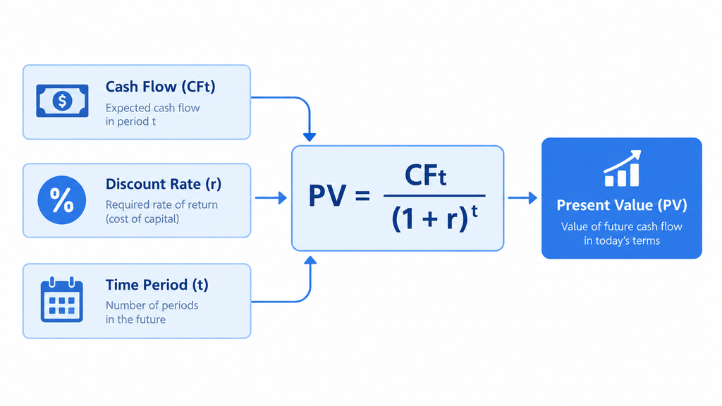
Breaking Down Each Variable

The cash flow variable represents the actual dollars a business is expected to generate in a given year, whether measured on an unlevered or levered basis for that specific model, an important point for anyone building financial models.

Discount rate meaning centers on compensation for both risk and the simple passage of time, where a higher rate signals greater uncertainty and a lower one reflects safer projected earnings, a detail that matters for accurate valuation work.

The time period simply counts which year of the forecast a specific cash flow belongs to, and this number feeds directly into the discount factor calculation for that year, which analysts must weigh carefully in practice.

Free Cash Flow to Firm (FCFF) vs. Free Cash Flow to Equity (FCFE)

FCFF, often called unlevered free cash flow, measures cash available to every capital provider, including both debt holders and shareholders, calculated before any interest payments are subtracted from totals, a factor that shapes the final valuation outcome.

FCFE, often called levered free cash flow, measures cash left specifically for common shareholders alone, after debt payments have already been accounted for within the company’s existing capital structure, something every serious financial analyst should understand well.

Choosing between FCFF vs FCFE depends on the valuation goal at hand. FCFF supports an enterprise value vs equity value approach for the whole firm, while FCFE targets shareholders directly, a nuance that affects how the model performs.

How to Calculate Discounted Cash Flow: Step-by-Step

Calculating discounted cash flow follows a repeatable sequence of steps that nearly any analyst can apply consistently, moving from initial cash flow forecasting through discount rate selection and beyond, which directly influences the credibility of the result.

Each stage in this valuation process builds directly on the last one, so accuracy early on really matters, since a weak growth rate assumption can distort every subsequent step in the model.

Most practitioners follow a five-step DCF walkthrough, moving from forecasting cash flows to discounting them and finally comparing the result against the current market price for context, a point worth remembering when reviewing any model.

The forecast period length typically spans five to ten years, depending heavily on industry stability and how predictable the company’s historical financials actually turn out to be over time, which can meaningfully change the final valuation figure.

Once all model building steps are finished, the valuation output becomes a single dollar figure per share or per company, which analysts then compare against current trading prices directly, an idea central to sound financial decision-making overall.

Step 1 Project Future Cash Flows

Cash flow forecasting begins with detailed revenue projections built from historical growth trends, prevailing market conditions, and management guidance where it happens to be publicly available for the business, a consideration that shapes how investors read the output.

Analysts then estimate operating cash flow by carefully adjusting projected earnings for non-cash items, working capital changes, and expected capital expenditures needed to sustain or meaningfully grow future operations, which underscores why careful assumptions matter so much.

These projections typically extend across a standard five-year forecast period, using historical financials as a reliable starting anchor while layering in reasonable growth assumptions for each individual year ahead, a factor analysts revisit throughout the modeling process.

Step 2 Determine the Discount Rate (WACC vs. Cost of Equity)

Discount rate selection depends heavily on which specific cash flow type is being valued in the model. Firm-level models typically use WACC, while equity-focused models rely on cost of equity, which helps explain differences across similar company models.

WACC blends together the cost of debt and cost of equity, weighted carefully by each financing source’s share of the overall capital structure weighting within the company’s total financing mix, an aspect that deserves close attention during review.

The chosen rate must reflect the required return investors demand given the business’s underlying risk profile, since a mismatched, overly optimistic risk-adjusted discount rate can quietly distort the entire output, an important point for anyone building financial models.

Step 3 Calculate the Terminal Value

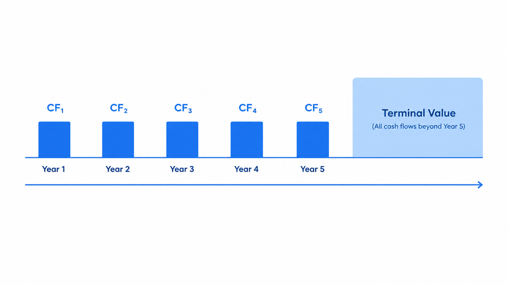
Terminal value captures the worth of every cash flow arriving beyond the explicit forecast horizon, since most healthy businesses are assumed to keep operating well past the model’s final projected year, a detail that matters for accurate valuation work.

Analysts typically choose between a perpetuity growth approach and exit multiple methods, depending on data availability and how the company is realistically expected to mature financially over time, which analysts must weigh carefully in practice.

This single figure, often labeled continuing value or residual value, frequently represents a surprisingly large share of total valuation, especially for younger, fast-growing companies with distant expected profitability, a factor that shapes the final valuation outcome.

Perpetuity Growth Method

The Gordon growth model assumes projected cash flows grow at one constant perpetuity growth rate forever after the forecast period ends, once the underlying business reaches a stable growth phase, something every serious financial analyst should understand well.

This terminal growth assumption should stay conservative and modest, often anchored near expected long-term GDP growth, since no single company can meaningfully outgrow the broader economy indefinitely without eventually slowing, a nuance that affects how the model performs.

Exit Multiple Method

The exit multiple method instead applies a comparable exit multiple, often based on observed EV/EBITDA multiple data drawn from similar companies, directly to the final projected year’s earnings figure, which directly influences the credibility of the result.

This approach produces a market-based terminal value firmly grounded in observable transaction multiple data, offering analysts a useful cross-check against the more theoretical perpetuity growth calculation described earlier in the model, a point worth remembering when reviewing any model.

Step 4 Discount and Sum Cash Flows to Find Present Value

Discounting cash flows simply means applying the appropriate discount factor per year to each projected amount, shrinking distant future cash flows more heavily than those arriving sooner in the timeline, which can meaningfully change the final valuation figure.

Analysts then calculate the sum of present values across the entire forecast period, combining every individually discounted year into one running total present value figure representing the business overall, an idea central to sound financial decision-making overall.

Finally, adding discounted terminal value to that running total produces the complete enterprise value calculation, representing the full estimated worth of the company’s expected future cash generation over time, a consideration that shapes how investors read the output.

Step 5 Interpret the Result (Undervalued vs. Overvalued)

Once the finished model produces a final number, analysts compare intrinsic value vs market price to see whether the current trading price sits meaningfully above or below that calculated figure, which underscores why careful assumptions matter so much.

If the calculated value exceeds the market price, the asset may appear an undervalued stock, suggesting the broader market has not fully recognized the company’s expected future cash generation potential, a factor analysts revisit throughout the modeling process.

Conversely, an overvalued stock signal appears whenever market price exceeds calculated intrinsic value. Analysts typically apply a margin of safety before treating any single result as a firm conclusion, which helps explain differences across similar company models.

Worked DCF Example (With Real Numbers)

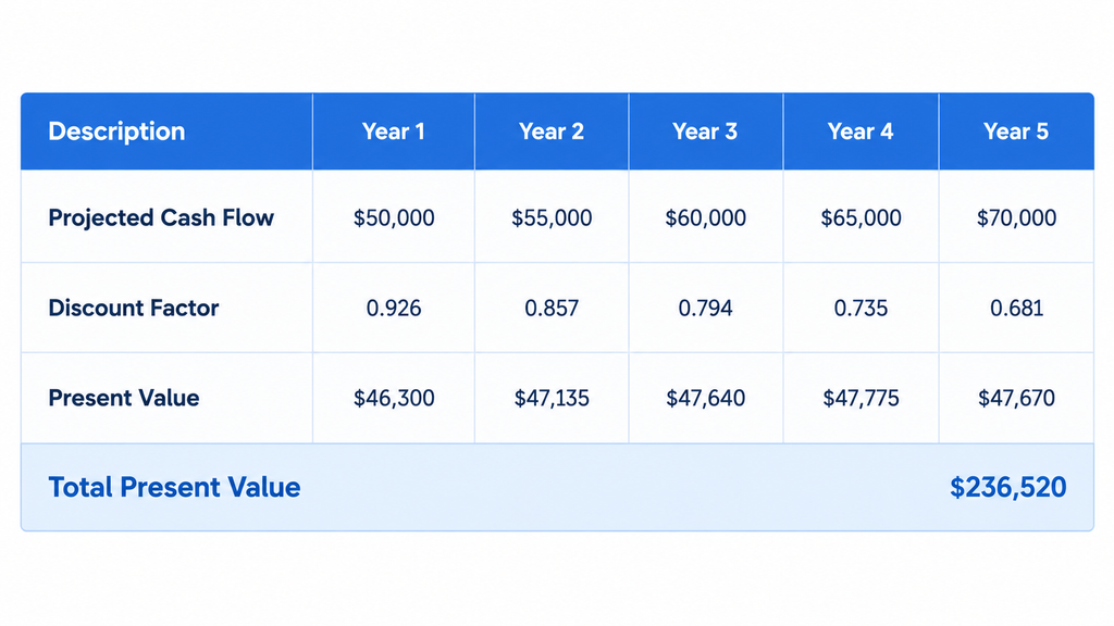
Consider a purely hypothetical company valuation, used only to illustrate the mechanics of a DCF example clearly, without representing any real business, industry, or actual set of published financial results, an aspect that deserves close attention during review.

Suppose this company generates a sample calculation cash flow of one hundred million dollars in year one, growing steadily across a five-year cash flow projection example before eventually reaching a stable phase.

Applying a discount rate example of ten percent, each year’s projected cash flow shrinks according to its own discount factor per year, producing a progressively smaller present value result for later years.

Summing those five separately discounted amounts, then adding a discounted terminal value example calculated through the perpetuity method, produces the complete valuation output example for this hypothetical illustrative business, an important point for anyone building financial models.

This practical DCF illustration shows how each formula component connects into one final number. Real-world models follow this exact same numerical structure, just with far more detailed inputs and assumptions, a detail that matters for accurate valuation work.

Building a DCF Model in a Spreadsheet

A working DCF Excel model typically separates inputs cleanly from outputs, keeping every assumption fully visible and easily editable within a dedicated input assumptions tab near the front of the workbook, which analysts must weigh carefully in practice.

This spreadsheet valuation structure usually includes a historical financials section, a forecast section, a discount rate calculation area, and a terminal value block, each one labeled and properly linked together, a factor that shapes the final valuation outcome.

Building a DCF model from scratch means starting with core revenue drivers, then flowing those numbers down through operating costs and capital spending until reaching projected free cash flow figures, something every serious financial analyst should understand well.

Good Excel formulas for DCF avoid hardcoded numbers wherever possible, instead referencing the input assumptions tab directly, which keeps the overall model structure flexible when assumptions inevitably need updating later, a nuance that affects how the model performs.

Finally, an output summary section consolidates the final valuation result, sensitivity ranges, and key assumptions onto one page, and this spreadsheet layout choice makes the whole valuation model setup easier to review.

Choosing the Right Discount Rate

The discount rate chosen for a DCF model directly shapes the final valuation output, since even small rate changes compound significantly across a multi-year forecast period and terminal value calculation, which directly influences the credibility of the result.

Most equity analysts calculate WACC when valuing an entire firm as a whole, blending both cost of equity and cost of debt according to each source’s weight in the financing structure, a point worth remembering when reviewing any model.

The risk-free rate, often based on long-term government bond yields, forms the foundation of the cost of equity calculation, before analysts add an equity risk premium for additional market risk exposure, which can change the final valuation figure.

Beta measures how much a particular stock’s returns move relative to the broader overall market, feeding directly into the CAPM formula alongside the risk-free rate and equity risk premium figures, an idea central to sound financial decision-making overall.

Ultimately, the weighted average cost of capital reflects the close relationship between risk and discount rate selection, meaning riskier businesses require higher rates to properly compensate investors for uncertainty, a consideration that shapes how investors read the output.

How to Calculate WACC

The WACC formula carefully weights the cost of debt and cost of equity by their respective shares of the company’s total market value of equity and debt combined together in the mix.

Because interest payments are generally tax-deductible, the cost of debt component includes a tax shield adjustment, reducing the effective borrowing rate below the company’s officially stated cost of debt slightly, which underscores why careful assumptions matter so much.

These weighted components ultimately combine into one single weighted cost of capital, following clear, well-established WACC calculation steps that most financial analysts and business students learn fairly early in training, a factor analysts revisit throughout the modeling process.

How Risk Affects the Discount Rate

A risk premium gets added on top of the risk-free rate whenever a company faces elevated company-specific risk, such as unstable earnings, high leverage, or significant customer concentration issues within operations, which helps explain differences across similar company models.

Industry risk also plays a meaningful role in this calculation, since some sectors face far more regulatory, cyclical, or technological uncertainty than others, justifying a higher discount rate for riskier cash flows.

This close relationship between risk and valuation explains why two seemingly similar companies can receive very different valuations. Discount rate sensitivity simply means small assumption changes can shift results substantially overall, an aspect that deserves close attention during review.

DCF vs. Other Valuation Methods

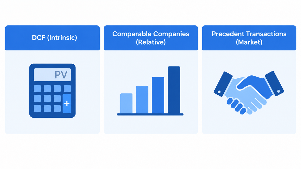
Valuation methods comparison typically places DCF alongside trading comps, precedent transactions, and dividend-based approaches, with each one offering a genuinely different lens for estimating what a business is actually worth, an important point for anyone building financial models.

DCF vs comparable company analysis highlights a core underlying distinction: intrinsic valuation looks inward at projected cash flows directly, while relative valuation looks outward at how similar peer companies currently trade, a detail that matters for accurate valuation work.

DCF vs precedent transactions raises a fairly similar contrast, since transaction-based multiples reflect actual deal prices paid by real buyers, rather than a purely theoretical estimate built from future projections alone, which analysts must weigh carefully in practice.

DCF vs dividend discount model matters for equity investors, since the dividend discount model focuses narrowly on distributed cash payments rather than total free cash flow generated by the business, a factor that shapes the final valuation outcome.

Understanding this broader valuation method selection process, including the strengths and weaknesses of each method, helps analysts choose an appropriate combination rather than relying on any single approach alone, something every serious financial analyst should understand well.

DCF vs. Comparable Company Analysis (Trading Comps)

Trading comps rely on observable market multiples, such as EV/EBITDA or price-to-earnings ratios, drawn from a defined peer group valuation set of similar publicly traded companies within the same industry, a nuance that affects how the model performs.

This relative valuation approach reflects current market sentiment quickly, but it can also inherit widespread mispricing if the entire peer group happens to be overvalued or undervalued together at once, which directly influences the credibility of the result.

The core comps vs intrinsic value distinction comes down to speed versus depth. Trading comps are faster to build, while DCF offers a far more detailed, assumption-driven picture of value, a point worth remembering when reviewing any model.

DCF vs. Precedent Transaction Analysis

Precedent transactions examine actual completed M&A comparable, using observed transaction multiples paid in prior acquisitions to estimate what a similar business might realistically be worth in a comparable deal today, which can meaningfully change the final valuation figure.

These multiples often include a meaningful control premium, reflecting the extra amount buyers typically pay to gain full operational control over a target company during a completed acquisition transaction, an idea central to sound financial decision-making overall.

This deal-based valuation approach works well within M&A contexts specifically, though available precedent data can sometimes be limited, dated, or difficult to compare across differing deal structures and terms, a consideration that shapes how investors read the output.

DCF vs. Dividend Discount Model (DDM)

The dividend discount model values a stock based solely on its expected future dividend payments, discounted carefully back to present value using an appropriate required rate of return over time, which underscores why careful assumptions matter so much.

DDM vs DCF becomes especially relevant for dividend-paying stocks with stable, predictable payout histories, where dividends closely track the company’s underlying free cash flow generation across most reporting periods, a factor analysts revisit throughout the modeling process.

For companies that reinvest heavily and pay little or no dividends at all, this equity valuation comparison favors DCF, since the Gordon growth model variant of DDM would meaningfully understate true value.

Advantages and Limitations of DCF Valuation

DCF advantages and DCF limitations both stem from the exact same core feature: the method relies heavily on forward-looking assumptions rather than observable current market prices or recent trading data, which helps explain differences across similar company models.

This forward-looking nature is precisely why DCF valuation remains popular among long-term investors, since it captures an intrinsic value focus rather than short-term price swings driven purely by sentiment alone, an aspect that deserves close attention during review.

At the same time, sensitivity to assumptions means results can vary widely depending on chosen growth rates, discount rates, and terminal value methodology selected carefully by the individual analyst involved, an important point for anyone building financial models.

Critics often summarize DCF’s core weakness with the phrase garbage in garbage out, meaning flawed inputs inevitably produce a flawed valuation, regardless of how sophisticated the underlying model complexity truly appears, a detail that matters for accurate valuation work.

Despite these real tradeoffs, understanding both the strengths of DCF and weaknesses of DCF helps analysts apply the method appropriately, rather than treating any single output as a certain guaranteed answer, which analysts must weigh carefully in practice.

Advantages

DCF valuation offers a genuine intrinsic value focus, meaning results are not dependent on market prices that can swing sharply due to sentiment, momentum, or short-term breaking news events in markets, a factor that shapes the final valuation outcome.

This makes the method especially flexible for private companies without any public trading price available, since valuation relies entirely on projected financial performance rather than observable, readily available market data, something every serious financial analyst should understand well.

Because building a DCF model requires genuinely detailed operational insight, the process itself often reveals valuable information useful for capital budgeting decisions and broader long-term strategic planning across the organization, a nuance that affects how the model performs.

Limitations and Common Pitfalls

Forecasting uncertainty grows substantially the further out projections extend into the future, since predicting revenue, margins, and capital needs a full decade ahead involves considerable subjectivity in inputs throughout, which directly influences the credibility of the result.

Discount rate sensitivity means even modest changes to WACC or cost of equity can shift the final valuation dramatically, sometimes by twenty percent or more depending on the specific inputs used, a point worth remembering when reviewing any model.

Terminal value overweighting is a genuinely frequent pitfall, since this single figure often represents most of total calculated value, making difficulty valuing early-stage companies particularly pronounced and challenging in practice, which can meaningfully change the final valuation figure.

Sensitivity Analysis: Stress-Testing Your DCF

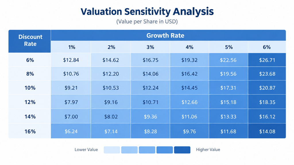
Sensitivity analysis tests how much the final valuation output changes when key underlying assumptions shift, helping analysts understand precisely which inputs matter most to the overall calculated result produced by the model.

Building a data table sensitivity grid, typically varying discount rate and terminal growth rate together across a range, shows a full DCF valuation range rather than one single fixed number output, an idea central to sound financial decision-making overall.

Scenario analysis extends this idea further by modeling a distinct best case worst case scenario, alongside a realistic base case, to capture a wide spread of possible future outcomes, a consideration that shapes how investors read the output.

This overall process produces a useful valuation confidence interval instead of false precision, openly acknowledging that every DCF output depends on assumptions rather than any guaranteed future outcome or result, which underscores why careful assumptions matter so much.

Ultimately, stress testing assumptions helps investors clearly understand the margin of error embedded within any single-point valuation estimate, encouraging a more cautious, measured interpretation of the final results produced, a factor analysts revisit throughout the modeling process.

DCF Valuation in Practice: Different Applications

DCF applications span far beyond public equities alone, extending meaningfully into valuing startups, valuing real estate, valuing private businesses, and broader project valuation work spanning many different industries and sectors, which helps explain differences across similar company models.

Industry-specific DCF use varies quite considerably, since capital-intensive sectors like utilities or real estate require noticeably different assumptions than asset-light software or service businesses currently being analyzed by an analyst, an aspect that deserves close attention during review.

These practical use cases appear consistently throughout DCF in investment banking, where analysts routinely build models supporting M&A advisory, fairness opinions, and capital raising transactions on a regular basis, an important point for anyone building financial models.

DCF in equity research similarly relies heavily on this method to generate reasonable price targets, supporting buy, sell, or hold recommendations published for both institutional and everyday retail investors alike, a detail that matters for accurate valuation work.

Across all these real-world DCF examples, the underlying mechanics stay remarkably consistent, even though specific assumptions, cash flow definitions, and chosen discount rates naturally shift depending on the particular context involved, which analysts must weigh carefully in practice.

Valuing Public Company Stocks

Stock valuation through DCF supports equity research analysts in building genuinely independent price targets, separate entirely from prevailing market sentiment or short-term trading momentum currently affecting the shares, a factor that shapes the final valuation outcome.

This process produces a defensible estimate of intrinsic stock value, which investors then compare against current trading prices before forming a broader, more informed buy sell hold decision framework for themselves, something every serious financial analyst should understand well.

Public company DCF models benefit greatly from abundant historical financials and existing analyst estimates, making this a genuinely common investor use case across both institutional and individual retail portfolios alike, a nuance that affects how the model performs.

Valuing Startups and Early-Stage Companies

Startup valuation presents distinctly unique challenges, since many early-stage companies report sustained negative cash flow for years before ever reaching sustainable profitability or consistently positive operating results overall, which directly influences the credibility of the result.

These early-stage DCF challenges stem largely from genuinely high uncertainty forecasting, since available historical data remains limited and future growth trajectories stay difficult to predict with any real reliability, a point worth remembering when reviewing any model.

Despite these real obstacles, venture valuation professionals still regularly apply modified DCF techniques for pre-revenue company valuation, often blending scenario analysis together with comparable transaction data drawn from similar deals, which can meaningfully change the final valuation figure.

Valuing Real Estate and Projects

Real estate DCF models carefully project rental income, ongoing operating expenses, and eventual sale proceeds, discounting each individual cash flow back using an appropriate required return figure over time, an idea central to sound financial decision-making overall.

This property income approach treats a building quite similarly to any other income-generating asset, projecting project cash flows across a defined holding period before the eventual final disposition occurs, a consideration that shapes how investors read the output.

Beyond real estate specifically, this broader project valuation work also supports general capital budgeting decisions, helping companies decide whether individual investments create sufficient long-term value for stakeholders overall, which underscores why careful assumptions matter so much.

Valuing Private Businesses and M&A Deals

Private company valuation relies especially heavily on DCF, since no public trading price exists at all to serve as an independent market reference point for meaningful comparison purposes, a factor analysts revisit throughout the modeling process.

This dependence makes DCF genuinely central to many M&A valuation processes, where both the buyer and seller each need an independent estimate before negotiating final transaction terms together, which helps explain differences across similar company models.

Because buyer and seller valuation perspectives often differ significantly from one another, DCF outputs frequently serve as a useful starting point for broader deal negotiation use case discussions between parties, an aspect that deserves close attention during review.

Common Mistakes to Avoid in DCF Valuation

One frequent DCF mistake involves applying an overly optimistic growth rate, extending unrealistic near-term growth trends far too deep into the forecast period without sufficient underlying business justification for that assumption, an important point for anyone building financial models.

Another common error is a mismatched discount rate and cash flow type, such as mistakenly applying WACC to equity-level cash flows instead of the technically correct cost of equity figure, a detail that matters for accurate valuation work.

Ignoring dilution from future planned share issuances can meaningfully overstate per-share value, especially for growth companies that regularly raise fresh capital through additional equity offerings over time, which analysts must weigh carefully in practice.

An unrealistic terminal value, often built on an unsustainable perpetual growth rate assumption, can silently dominate the entire valuation output, masking otherwise weaker near-term forecast assumptions underneath the surface, a factor that shapes the final valuation outcome.

Following a clear, disciplined model checklist and established best practices for accuracy helps analysts catch these common forecasting errors and other common valuation errors before finalizing any published results, something every serious financial analyst should understand well.

Frequently Asked Questions

What is a good discount rate to use in a DCF model?

An appropriate discount rate depends heavily on company-specific risk, industry, and existing capital structure, meaning no single universal number applies equally well across every possible business or valuation scenario imaginable, a nuance that affects how the model performs.

Many analysts start with a WACC benchmark reflecting a typical discount rate range for the relevant industry, then adjust upward for company-specific or industry discount rate risk factors as needed, which directly influences the credibility of the result.

Is DCF the same as NPV?

DCF vs NPV are closely related concepts but not technically identical. Net present value typically subtracts an initial investment cost from total discounted cash flows, producing one final net figure, a point worth remembering when reviewing any model.

DCF, by contrast, often refers to the broader overall valuation process itself. Both concepts nonetheless share the exact same underlying capital budgeting terminology and discounting mathematics throughout their calculations, which can meaningfully change the final valuation figure.

What are the biggest weaknesses of DCF valuation?

The most significant DCF limitations include persistent forecasting uncertainty over long time horizons and heavy terminal value risk, since this single figure often dominates the entire total valuation result, an idea central to sound financial decision-making overall.

Assumption sensitivity also raises legitimate concerns about overall model reliability, since even small changes to growth or discount rate inputs can shift the final valuation result quite substantially, a consideration that shapes how investors read the output.

How many years should a DCF forecast period cover?

Forecast period length commonly ranges from five to ten years total, depending on how predictable the underlying business is and how quickly it approaches a genuinely stable growth phase overall, which underscores why careful assumptions matter so much.

The choice between a 5-year vs 10-year forecast ultimately depends on industry maturity, since the explicit forecast horizon should ideally end once growth rates naturally normalize over time, a factor analysts revisit throughout the modeling process.

Can DCF be used to value a company with negative cash flow?

Yes, though negative free cash flow complicates the overall process considerably. This situation represents a common startup valuation challenge for pre-profitability company situations lacking any established earnings history, which helps explain differences across similar company models.

Analysts typically address this issue through alternative valuation approach blending, combining longer early-stage forecasting windows with scenario analysis to capture a genuinely wider range of possible outcomes, an aspect that deserves close attention during review.

What’s the difference between DCF and comparable company analysis?

The core underlying distinction is intrinsic vs relative valuation. DCF builds value carefully from projected fundamentals, while trading comps comparison relies instead on how similar companies currently trade in markets, an important point for anyone building financial models.

This reflects a broader market-based valuation versus fundamentals-based split overall, and understanding these valuation method differences helps analysts choose the right tool for each particular situation they face, a detail that matters for accurate valuation work.

How accurate is DCF valuation?

Valuation accuracy depends heavily on assumption dependency throughout the model, since even carefully well-built models can suffer meaningful forecasting error if growth or margin projections prove incorrect later on, which analysts must weigh carefully in practice.

Because of this inherent uncertainty, analysts often apply a margin of safety and present results as a sensitivity range rather than presenting one single, falsely precise number to readers, a factor that shapes the final valuation outcome.

What is terminal value and why does it matter so much in DCF?

Terminal value importance stems directly from its sheer size. It frequently represents a large percentage of total valuation, sometimes exceeding half of the entire calculated result on its own, something every serious financial analyst should understand well.

Both perpetuity growth impact and exit multiple impact significantly influence overall valuation weighting, making terminal value assumptions among the single most important choices in building any working model, a nuance that affects how the model performs.

Should I use FCFF or FCFE in my DCF model?

The FCFF vs FCFE choice ultimately depends on your specific valuation goal at hand. FCFF supports a broader enterprise value approach covering the whole firm, including both debt and equity holders together.

FCFE instead supports a direct equity value approach, making capital structure consideration especially important when deciding which method produces the most accurate final valuation output difference for your purposes, which directly influences the credibility of the result.